Black Variance Surface in PyQL

Summary: Building Black Variance Surfaces in PyQL

In my previous post on Variance Swaps, I neglected to mention an important implementation detail. If you look the Variance Swap unittest or example script you'll see that replicating pricer requires a BlackVarianceSurface object. I had to build bindings for these in PyQL so I thought I'd mention how they work.

BlackVarianceSurface is a volatility termstructure that implements different types of 2-d interpolation routines between implied volatility quotes. I included two types of interpolations from the Quantlib source code:

• Bilinear
• Bicubic

To over simplify, Bilinear linearly interpolates between neighboring quotes. Bicubic uses a cubic spline routine (third order polynomial) to smoothly interpolate between points.

See for wikipedia for a nice summary of the differences between bicubic vs. bilinear interpolation.

The python interface is given in the example below

Copycopy code to clipboard
1...
2dc = Actual365Fixed()
3calendar = UnitedStates()
4
5calculation_date = Date(6, 11, 2015)
6
7spot = 659.37
8Settings.instance().evaluation_date = calculation_date
9
10dividend_yield = SimpleQuote(0.0)
11risk_free_rate = 0.01
12dividend_rate = 0.0
13# bootstrap the yield/dividend/vol curves
14flat_term_structure = FlatForward(
15    reference_date=calculation_date,
16    forward=risk_free_rate,
17    daycounter=dc
18)
19
20flat_dividend_ts = FlatForward(
21    reference_date=calculation_date,
22    forward=dividend_yield,
23    daycounter=dc
24)
25
26dates = [
27    Date(6,12,2015),
28    Date(6,1,2016),
29    Date(6,2,2016),
30    Date(6,3,2016),
31]
32
33strikes = [527.50, 560.46, 593.43, 626.40]
34
35data = np.array(
36    [
37        [0.37819, 0.34177, 0.30394, 0.27832],
38        [0.3445, 0.31769, 0.2933, 0.27614],
39        [0.37419, 0.35372, 0.33729, 0.32492],
40        [0.34912, 0.34167, 0.3355, 0.32967],
41        [0.34891, 0.34154, 0.33539, 0.3297]
42    ]
43)
44
45vols = Matrix.from_ndarray(data)
46
47# Build the Black Variance Surface
48black_var_surf = BlackVarianceSurface(
49    calculation_date, NullCalendar(), dates, strikes, vols, dc
50)
51
52strike = 600.0
53expiry = 0.2 # years
54
55# The Surface interpolation routine can be set below (Bilinear is default)
56black_var_surf.set_interpolation(Bilinear)
57print("black vol bilinear: ", black_var_surf.blackVol(expiry, strike))
58black_var_surf.set_interpolation(Bicubic)
59print("black vol bicubic: ", black_var_surf.blackVol(expiry, strike))

As a sanity checked, I re-implemented results from an excellent blog post by Gouthaman Balaraman. In that post, the author builds a BlackVarianceSurface object using Quantlib's swig bindings.

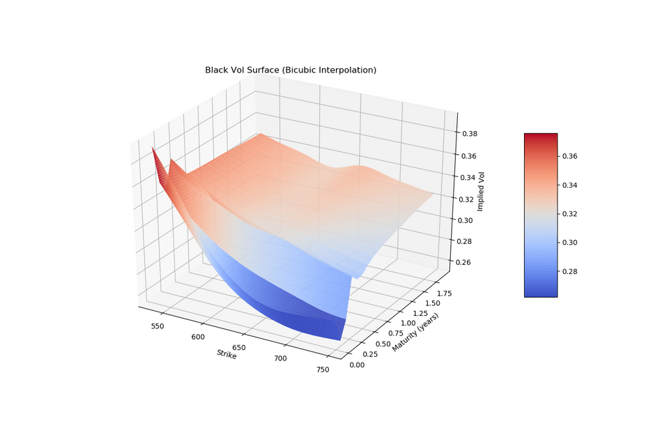
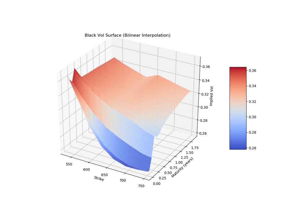
The plots for the same market data are given below:

For Bilinear interpolation, the surface looks like

For Bicubic interpolation, the surface looks like

As you can see from the plots, the bicubic is slightly smoother than bilinear.

Take a look at the PyQL bindings on my github page to see how the BlackVarianceSurface is implemented. The script to generate the plots is here

One thing that I clearly need to improve is the flexibility on the volatility data structure input to the BlackVarianceSurface constructor. It would be better to allow the vols data structure to be either a list of lists, a numpy array, or a QL Matrix object. I'll try to fix that at some point.

See you next time.