Local Volatility in PyQL

04.01.2020 — QuantLib — 1 min read

Summary: Local Volatility Surface in PyQL

Following on my previous post, I wanted to review the important concept of Local Volatility. Many books and articles 1, 2 are dedicated to discussing this topic. I won't go into great detail here, I just want to give a basic overview along with implementation details in PyQL.

Essentially, the idea of Local Volatility is to identify a level-dependent diffusion that exactly reproduces market implied volatilities. The contribution of Dupire was to prove that this diffusion is unique while also providing a convenient technique for deriving it from market quotes.

The full derivation of the local volatility function is given in section 2.2 and the appendix of 2. Here, I'll just give a sketch of the approach.

To begin, consider a generic, level-dependent, 1-D Brownian motion

\frac{\partial S}{S} = \mu(t, S)\partial t + \sigma(t,S)\partial W

Note that, the volatility for this process is not itself stochastic. We can use this process to model the diffusion on a equity spot price in the presence of a short rate $r(t)$ and a dividend yield $D(t)$ . A European call option for this process then satisfies a modified version of the Black-Scholes equation:

\frac{\partial{C}}{\partial{t}} = \frac{\sigma^2K^2}{2}\frac{\partial^2C}{\partial K^2} + (r(t) - D(t))\left(C- K\frac{\partial{C}}{\partial{K}}\right)

We can simplify this equation by writing $C(S_0, K,T)$ as a function of the forward price $F_T=S_0\exp(\int_0^T\mu(t)dt) = S_0\exp(\int_0^T(r(t) - D(t))dt)$ , (i.e. use the forward measure)

In these units, Black-Scholes equation simplifies to

\frac{\partial C}{\partial t} = \frac{\sigma^2K^2}{2}\frac{\partial^2 C}{\partial K^2}

or solving for the volatility gives Dupire's equation

\sigma^2(K,T) = \frac{\frac{\partial C}{\partial T}}{\frac{1}{2}K^2\frac{\partial^2 C}{\partial K^2}}

Market quotes are usually given in terms of Black-Scholes implied volatilities. We can express the local volatility in terms of these quantities by equating the price equations for the two models

C_{local}(S_0, K,T) = C_{BS}(S_0, K, \sigma_{BS}, T)

The strategy is then to solve for the local volatility in terms of the Black-Scholes impliedvolatility since we have a closed form expression for the $C_{BS}$ . The full derivation is given in section 2.2 of 2 . Here we just reproduce the results.

Namely, using more convenient units, the Black-Scholes total variance

w(S_0,K,T) = \sigma^2_{BS}(S_0,K,T)T

and log-moneyness $y = \ln\left(\frac{K}{F_T}\right)$

We can show that the local variance $v_{local} = \sigma^2(S_0, K,T)$

satisfies the following expression:

v_{local} = \frac{\frac{\partial w}{\partial T}}{1 - \frac{y}{w}\frac{\partial w}{\partial y} + \frac{1}{4}\left(-\frac{1}{4} - \frac{1}{w} + \frac{y^2}{w^2}\right)\left(\frac{\partial w}{\partial y}\right)^2 + \frac{1}{2}\left(\frac{\partial^2 w}{\partial y^2}\right)}

Quantlib implements this equation in ql.termstructure.volatility.equityfx.localvolsurface

In the code excerpt below we, show the LocalVolSurface is used in PyQL. It follows a similiar interface and BlackVarianceSurface given in the previous post.

1calc_date = Date(6, 11, 2015)
2Settings().evaluation_date = calc_date
3
4risk_free_rate = 0.01
5dividend_rate = 0.0
6
7day_count = Actual365Fixed()
8calendar = UnitedStates()
9
10flat_ts = FlatForward(calc_date, risk_free_rate, day_count)
11dividend_ts = FlatForward(calc_date, dividend_rate, day_count)
12
13expiration_dates = [
14    Date(6,12,2015),
15    Date(6,1,2016),
16    Date(6,2,2016),
17    Date(6,3,2016),
18    Date(6,4,2016)
19]
20
21strikes = [527.50, 560.46, 593.43, 626.40]
22
23data = np.array(
24    [
25        [0.37819,0.34450,0.37419,0.37498,0.35941],
26        [0.34177,0.31769,0.35372,0.35847,0.34516],
27        [0.30394,0.29330,0.33729,0.34475,0.33296],
28        [0.27832,0.27614,0.32492,0.33399,0.32275]
29    ]
30)
31
32vols = Matrix.from_ndarray(data)
33
34black_var_surf = BlackVarianceSurface(calc_date,
35                                      calendar,
36                                      expiration_dates,
37                                      strikes,
38                                      vols,
39                                      day_count)
40
41spot = 659.37
42strike = 600.0
43expiry = 0.2 # years
44
45local_vol_surf = LocalVolSurface(black_var_surf,
46                                 flat_ts,
47                                 dividend_ts,
48                                 spot)
49
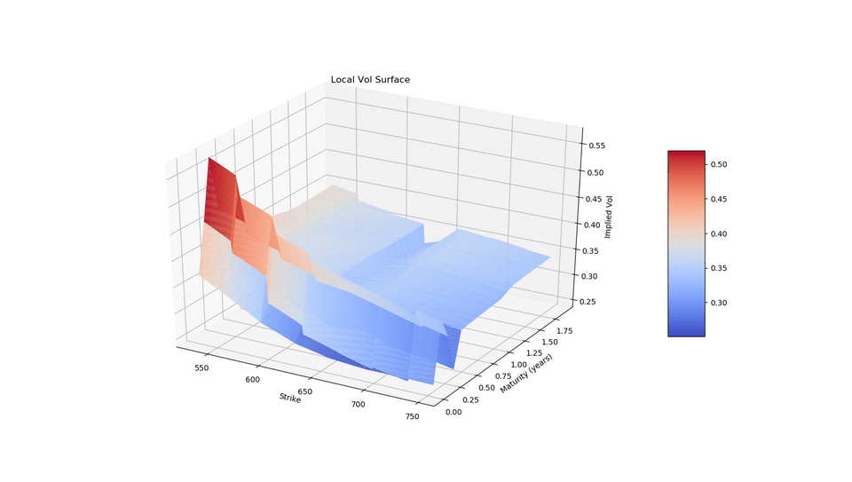
50print("local vol: ", local_vol_surf.localVol(expiry, strike))

In the plots below, we can see what the LocalVolSurface looks like:

Take a look at the PyQL bindings on my github to see an example of the LocalVolSurface. See you next time.