Simulating the Heston Process

29.04.2018 — Numerical Methods, QuantLib — 3 min read

Summary: We investigate different discretization schemes for the Heston Process, looking at issues of numerical bias and ease of implementation

In today's post, I will examine a few issues related to numerical simulation of the Heston model. As a quick reminder, the Heston process is a stochastic volatility model defined by the following sde:

dS_t = (r-d) S_t dt + \sqrt{V_t} S_t dW^s_t

dV_t = \kappa (\theta - V_t) dt + \sigma \sqrt{V_t} dW^\upsilon_t

dW^s_t dW^\upsilon_t = \rho dt

for asset price $S_t$ . $dW_t^s$ and $dW_t^{\nu}$ are Wiener processes with correlation $\rho$ . As usual, $r$ and $d$ are the risk free and dividend rates respectively.

The Heston model is an excellent benchmarking model due to the surprising fact that it's probability distribution function (pdf) has a closed formed expression. It's a one of five such processes in 1 or 2 dimensions PHL. With the closed form pdf, we can easily compare the performance of the Heston model's numerical simulation by comparing PV's of a Monte Carlo pricer with an analytic pricer.

To carry out a numerical simulation we first need to choose a discretization scheme. That is, we need to approximate the infinitesimal diffusion process with a finite scheme to be used in the simulation code. Any such scheme may potentially introduce bias into the simulation that could alter the realized moments of the pdf.

The simplest possible scheme is a first order expansion, i.e. an Euler Mayorana (or just ''Euler'') scheme. Transforming to $\ln S$ and discretizing $t$ to step size $\Delta$ gives

\ln S(t + \Delta) = \ln S(t) + \left(r - d - \frac{1}{2}V(t)\right)\Delta +\sqrt{V(t)} Z_S\sqrt{\Delta}

V(t + \Delta) = V(t) + \kappa\left(\theta - V(t)\right)\Delta + \sigma \sqrt{V(t)} Z_V \sqrt{\Delta}

However, it turns out that this scheme does introduce bias. Furthermore, in this scheme it's possible to drive the variance process to negative values, which is outside the range of the pdf and causes the simulation to stop as $\sqrt{V}$ becomes imaginary.

One immediate fix to this problem is the floor V at 0, giving the so called "Truncated" scheme. Other schemes are based on higher order expansions of the sde or utilizing the closed form expression for the pdf. These are documented extensively in the literature Anderson. We list some of the schemes below

Euler Mayorana
Truncated
Quadratic Exponential
Broadie Kaya (Exact Simulation)

Broadie Kaya is based off direct sampling from the pdf but is rather difficult to implement numerically. The Quadratic Exponential (developed in Anderson) approximates the pdf using simplified functions and moment matching. The pdf for high and low values of the variance are matched against two different functions and threshold is implemented to switch between the two functions during a diffusion. This technique allows one to minimize variance while also easing the numerical implementation. As such, this scheme it is often the preferred scheme for Heston simulations.

QuantLib Implementation

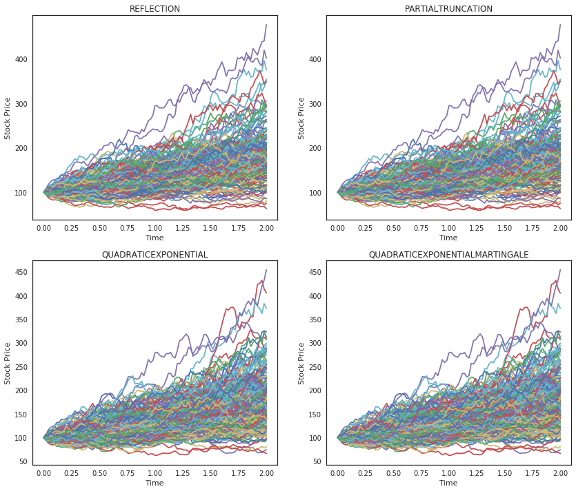
QuantLib includes several of these discretization schemes in their Heston Process class. Let's see what a simulation looks like.

Quick note: Although the HestonProcess class is available through the SWIG bindings, it does not expose the discretizations argument. Instead, we use PyQL, which has all the discretizations available.

1from quantlib.processes.heston_process import *
2from quantlib.quotes import SimpleQuote
3from quantlib.settings import Settings
4from quantlib.termstructures.yields.flat_forward import FlatForward
5from quantlib.time.api import today, TARGET, ActualActual, Date, Period, Years
6from quantlib.models.equity.heston_model import (HestonModel,
7                                                 HestonModelHelper)
8from quantlib.pricingengines.api import (AnalyticHestonEngine)
9from quantlib.pricingengines.vanilla.mceuropeanhestonengine import MCEuropeanHestonEngine
10from quantlib.instruments.api import (PlainVanillaPayoff,
11                                      EuropeanExercise,
12                                      VanillaOption,
13                                      EuropeanOption)

Defining the Heston Process

1def flat_rate(forward, daycounter):
2    return FlatForward(
3        forward = forward,
4        settlement_days = 0,
5        calendar = TARGET(),
6        daycounter = daycounter
7    )
8
9settings = Settings.instance()
10settlement_date = today()
11settings.evaluation_date = settlement_date
12
13day_counter = ActualActual()
14interest_rate = 0.7
15dividend_yield = 0.4
16
17risk_free_ts = flat_rate(interest_rate, day_counter)
18dividend_ts = flat_rate(dividend_yield, day_counter)
19
20maturity = Period(10, Years)
21exercise_date = settlement_date + maturity
22
23# spot
24s0 = SimpleQuote(100.0)
25
26# Available descritizations
27#PARTIALTRUNCATION
28#FULLTRUNCATION
29#REFLECTION
30#NONCENTRALCHISQUAREVARIANCE
31#QUADRATICEXPONENTIAL
32#QUADRATICEXPONENTIALMARTINGALE
33#BROADIEKAYAEXACTSCHEMELOBATTO
34#BROADIEKAYAEXACTSCHEMELAGUERRE
35#BROADIEKAYAEXACTSCHEMETRAPEZOIDAL
36
37# Heston Model params
38v0 = 0.05
39kappa = 5.0
40theta = 0.05
41sigma = 1.0e-4
42rho = -0.5
43
44def gen_process(desc):
45    process = HestonProcess(risk_free_ts,
46                            dividend_ts,
47                            s0,
48                            v0,
49                            kappa,
50                            theta,
51                            sigma,
52                            rho,
53                            desc)
54    return process
55
56processes = {
57  "REFLECTION" : gen_process(REFLECTION),
58  "PARTIALTRUNCATION" : gen_process(PARTIALTRUNCATION),
59  "QUADRATICEXPONENTIAL" : gen_process(QUADRATICEXPONENTIAL),
60  "QUADRATICEXPONENTIALMARTINGALE" : gen_process(QUADRATICEXPONENTIALMARTINGALE),
61}

Visualizing the Simulation

Note: The simulate function is not part of Quantlib. It has been added to the PyQL interface (see folder quantlib/sim).

1from quantlib.sim.simulate import simulate_process
2from quantlib.time_grid import TimeGrid

1import pandas as pd
2import numpy as np
3import matplotlib.pyplot as plt
4%matplotlib inline
5import seaborn as sns
6sns.set(style="white", rc={"axes.facecolor": (0, 0, 0, 0)})

1# simulate and plot Heston paths
2paths = 200
3steps = 100
4horizon = 2
5seed = 154
6
7grid = TimeGrid(horizon, steps)
8
9fig, axs = plt.subplots(figsize=(14, 12), nrows=2, ncols=2)
10flat_axs = axs.reshape(-1)
11
12for i, key in enumerate(processes.keys()):
13    flat_axs[i].plot(list(grid), simulate_process(processes[key], paths, grid, seed))
14    flat_axs[i].set_xlabel('Time')
15    flat_axs[i].set_ylabel('Stock Price')
16    flat_axs[i].set_title('%s' % key)

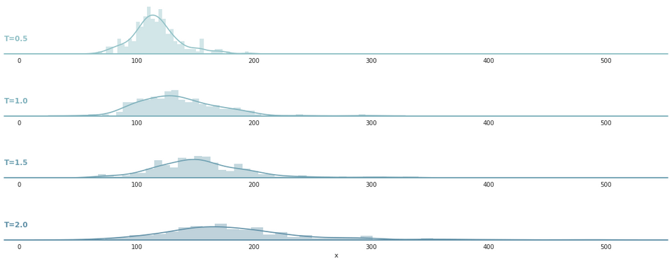
Let's look at of the diffusions in detail, for example the evolution of the Heston process using Partial Truncation looks like this

1res = simulate_process(processes["PARTIALTRUNCATION"], paths, grid, seed)
2x = res[[25,50,75,100],:].reshape(4*paths)
3
4g = np.repeat(["T=0.5","T=1.0","T=1.5","T=2.0"], paths)
5df = pd.DataFrame(dict(x=x, g=g))
6
7# Initialize the FacetGrid object
8pal = sns.cubehelix_palette(10, rot=-.25, light=.7)
9g = sns.FacetGrid(df, row="g", hue="g", aspect=10, size=1.6, palette=pal)
10
11g.map(sns.distplot, "x", bins=40, kde=True, rug=False)
12g.map(plt.axhline, y=0, lw=2, clip_on=False)
13
14
15def label(x, color, label):
16    ax = plt.gca()
17    ax.text(0, .3, label, fontweight="bold", color=color,
18            ha="left", va="center", transform=ax.transAxes)
19
20g.map(label, "x")
21g.fig.subplots_adjust(hspace=.25)
22g.set_titles("")
23g.set(yticks=[])
24g.despine(bottom=True, left=True)

Comparing the PV's of different engines

To examine the performance of the numerical schemes, we simply compare the PV's the same Call Option priced with an analytic and Monte Carlo engine. The results for different time steps and schemes are given in the table below

1# Build a Call Option
2payoff = PlainVanillaPayoff('Call', 105)
3exercise = EuropeanExercise(exercise_date)
4option = EuropeanOption(payoff, exercise)
5
6results = {"REFLECTION" : [],
7           "PARTIALTRUNCATION" : [],
8           "QUADRATICEXPONENTIAL" : [],
9           "QUADRATICEXPONENTIALMARTINGALE" : [],
10}
11
12# steps per year
13steps = [1, 4, 8, 16]
14
15for k, v in processes.items():
16    for step in steps:
17        mc_engine = MCEuropeanHestonEngine(v,
18                                           steps_per_year=step,
19                                           required_samples=500,
20                                           seed=1234,
21                                           )
22        option.set_pricing_engine(mc_engine)
23        results[k].append((np.around(option.npv, 5), np.around(option.error_estimate, 5)))
24
25
26results["time steps per year"] = steps
27results_df = pd.DataFrame(data = results)
28cols = results_df.columns.tolist()
29cols = cols[-1:] + cols[-2:-1] +  cols[:-2]
30results_df = results_df[cols]

1results_df

time steps per year	REFLECTION	PARTIAL TRUNCATION	QUADRATIC EXPONENTIAL	QUADRATIC EXPONENTIAL MARTINGALE
1	(1.64404, 0.05392)	(1.74109, 0.03607)	(1.71144, 0.02744)	(1.71527, 0.02811)
4	(1.64447, 0.06608)	(1.74109, 0.03607)	(1.71144, 0.02744)	(1.71527, 0.02811)
8	(1.98966, 0.04768)	(1.77399, 0.03692)	(1.70905, 0.02727)	(1.73049, 0.02829)
16	(1.80227, 0.03563)	(1.75864, 0.0351)	(1.70581, 0.02687)	(1.72956, 0.02818)

Conclusion

As we saw, there are many ways to simulate the Heston model, each with strengths and weaknesses with regards to bias/accuracy and runtime performance. In general, the Quadratic Exponential scheme performed better than Euler-type schemes, especially for simulations with fewer time steps per year.

In a future post, I will visit the local stochastic volatility version of the Heston model to see how it's simulation works.

Is there a better way?

If you take a look at the HestonProcess class file in QuantLib you will see that it, for each discretization, there is a different diffusion implementation. The user chooses the discretization from an enumerated list. The downside to this approach is that , in addition to creating bloated code, the list is always finite. What happens when someone wants to create a new discretization scheme that's not on the list? She has to add the diffusion implementation directly into the HestonProcess class.

A better approach might be to allow the user to build her own discretization in Python and then "compile-down" to C++ in the similar way to how the finite difference stencils are created in Devito [see my earlier post] This may just be hopeful speculation on my part :). Until next time.